- Introduction to the cleverMachine suite
- Internal workings
- Output interpretation
- Sample Datasets
- System requirements
Introduction to the cleverMachine suite
Experimentalists are nowadays increasingly faced with dealing with bioinformatics, especially sequence-based data. Many of the existing tools can be hard to use for untrained users, rendering them effectively unavailable to large number of people. Being able to extract information from datasets without the need to, for example, use a command line, can be extremely useful. We aim to develop such tools. With the cleverMachine suite, we to extend our toolkit with a general signal-detection and analysis tools for protein datasets.
Internal workings
The tool examines two datasets of protein sequences. For interpretation purposes, one of them is thought of a signal dataset and the other as a reference. The tool then creates protein signatures for each of the proteins, utilising a large set of protein scales - both experimentally derived and statistically derived from other tools' outputs. The protein signatures are then compared and combined to determine what features have the datasets in common, or more importantly, which ones are distinct for the individual sets.
Input data
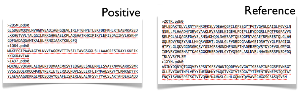
As was mentioned before, the whole story begins with two protein datasets. One of them will be considered a positive dataset and the other a negative. This is purely for interpretation purposes and, as we will see later, does not introduce any bias in the decision.
One may ask - why the need of a reference for signal detection? Our algorithm is unique in a way that it does not use any explicit scoring or parametrisation to derive its main result. It analyses both datasets only with relation to one another and thus a reference is essential.
The variables at play
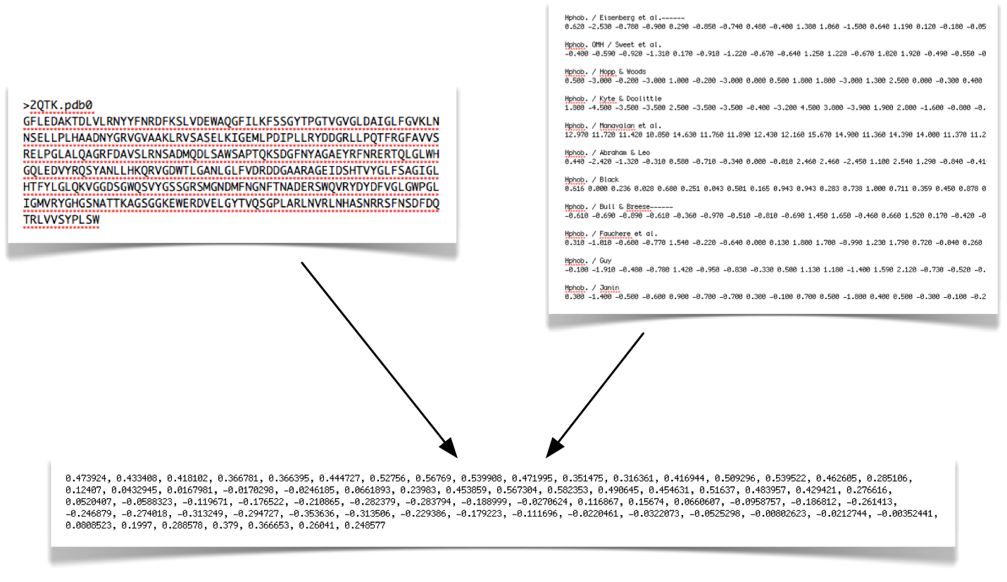
The very first step of algorithm operation is information extraction from protein sequences. A number of experimental scales (shown top right) are applied to individual protein sequences. Each amino acid (AA) in the sequence is then scored and turned into a profile:
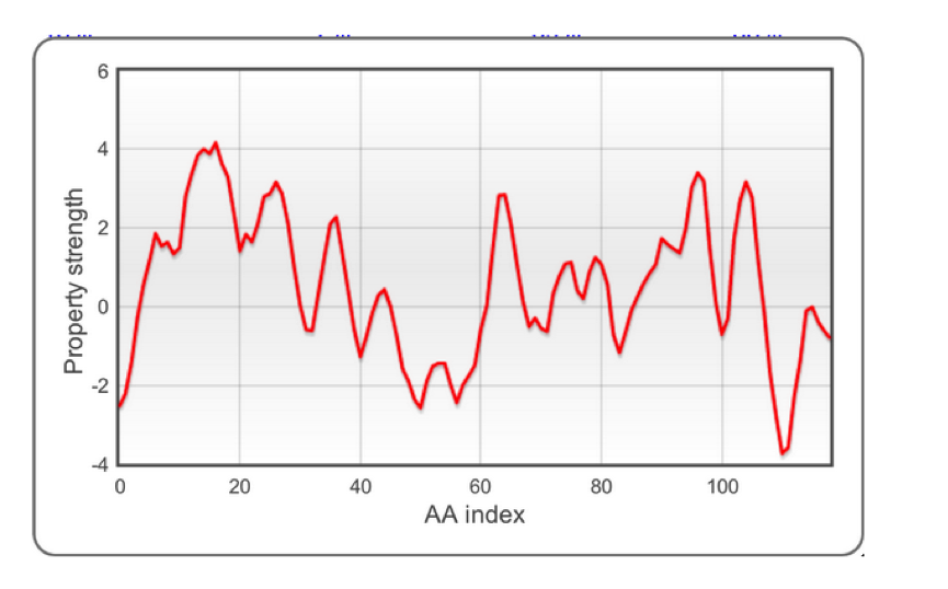
The raw profiles are processed and smoothed to clean up noise. Please note that the values range is as in the original publications (data are not normalized). After this step, a large amount of information is ready for statistical analysis.
Comparison steps
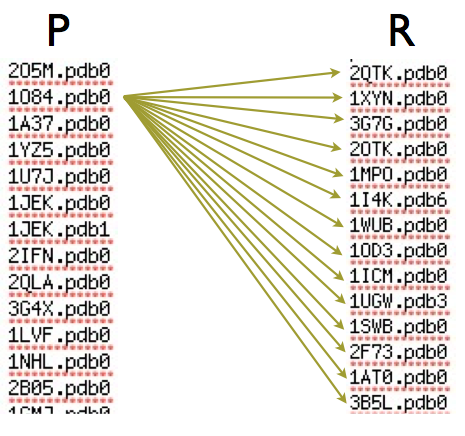
The method then looks for similarities and differences between individual proteins versus the other dataset. The example shown on the right hand side (RHS) shows the process being done for one of the elements of the positive dataset. The property strength for the individual is compared to each of the elements of the other dataset and if it significantly differs (in more than 75% of cases), the protein gets selected. This is repeated for each protein, each scale and each dataset, leading to creation of relative strength statistics.
Final processing
The final processing is the step where the real data crunching begins. The simple comparison results are collated and shown to the user and then a series of combination steps is created to determine which properties are most prominent on the dataset.
Signal strength detection
But, before any of the above may take place, feasiblity of the analysis is determined. Signal strength is determined by taking multiple samplings of both of the datasets and running analysis between them. The main hypothesis is that if the property is there in the dataset, mixing the datasets together should diminish, or altoghether remove, any information.
Strenght of any information is compared to the backgroudn noise generated from the user's provided data, leading to a reliable indicator of property strength. Only properties that qualify are considered for the further analytical steps.
Classification model evaluation
Available models include support vector machine, tree classifiers and adaptive boosting algorithms. The cleverMachine evaluates which of the classifier types performs best on the training set (using 10-fold cross validation) and the most accurate algorithm is chosen.
Output interpretation
Please see the tutorial section of the documentation.
Sample Datasets
To test the tool without availability of any datasets, we have provided datasets which are ready to be submitted
into our system via just a few clicks.
Just select a sample dataset on the new submission page.
Expert mode
The expert mode unleashes CM for the advanced user and provides more access to the internal workings
of the tool and multitude of calculation options.
However, this extra power does come with responsibility, which in this case is shifted
solely to the user. For example, when custom scales are uploaded, the become part
of the scale list, leaving the user responsible to make sure that consistency contraints hold.
Cross-validation of coverages
In the expert mode, the coverages in the individual scale view represent cross-validated result, where the input sets are sampled multiple times to provide a measure of internal set consistency. A visual illustration of the dependcy is provided in a form of linked plot. In the expert mode, the coverage of each individual scale is computed using a 5-fold cross validation (i.e., 4/5 of the datasets are used for training and 1/5 for testing). Cross-validation performances are reported in a plot.
Derived scale
Another perquisite of the expert mode is generation of a custom "scale" that is based on the difference of amino-acid counts between the input sets normalised by their occurences. It can be downloaded from the output page and used with further submissions.
Custom scales upload
The custom scale upload facility allows submission of user-provided scales. A popular and comprehensive source of scale files is for example http://www.genome.jp/aaindex/. Before the scale can be used with the CM, it needs to conform to a following file format:
- Line 1: Scale title - any text identifying the scale
- Line 2: amino-acid mappings. This is a space-separated values for each of the 20 amino acids in the following order:
A R N D C Q E G H I L K M F P S T W Y V
- The above can repeat for up to 10 custom scales and the scales do not need to be normalised.
For example, here are contents of a file representing two custom scales:
Signal sequence helical potential (Argos et al., 1982)
1.18 0.20 0.23 0.05 1.89 0.72 0.11 0.49 0.31 1.45 3.23 0.06 2.67 1.96 0.76 0.97 0.84 0.77 0.39 1.08
Membrane-buried preference parameters (Argos et al., 1982)
1.56 0.45 0.27 0.14 1.23 0.51 0.23 0.62 0.29 1.67 2.93 0.15 2.96 2.03 0.76 0.81 0.91 1.08 0.68 1.1
Variable threshold calculation
Normal CM submission uses coverage (see above) threshold of 0.75, determined to be the optimal for both high and low signal cases. The variable thershold calculation option looks through a set of thresholds to determine the very best one for a particular case. This is done at expense of a computation time and submissions will take longer to process.
Information extraction mode
Traditional CM uses invidiual averages of whole protein profiles to represent and compare them. We are aware that using a global measure for each of the proteins can lead to a loss of information as peaks can be masked by large areas with little signal. We are working to support additional means of information extraction and our first attempt is a peak-detecting approach. It filters out areas insignificant (closer than one standard deviation to a global property mean) and only considers large positive peaks. It should be noted that this is constantly evolving feature and any results obtained may be subject to change without notice.
System requirements
The tool's result can in theory be viewed in any modern browser, however, it is only fully tested in following browsers:
- latest version of Google Chrome
- latest version of Mozilla Firefox
If you experience any problems, please first try updating your browser to the latest version. The only version of the Internet Explorer that is theoretically capable of displaying the result is 10, the latest at the time of writing.